
This is an optional read for the 5 part series I wrote on learning parameters. In this post, you will find some basic stuff you’d need to understand my other blog posts on how deep neural networks learn their parameters better. You can check out all the posts in the Learning Parameters series by clicking on the kicker tag at the top of this post.
We will briefly look at the following topics:
A multivariable function is just a function whose input and/or output is made up of multiple numbers/variables. E.g., f(x, y) = z= x² + y².
Functions with multiple outputs are also called multivariable functions, but they are irrelevant here.
The term “gradient” is just a fancy way of referring to derivatives of multivariable functions. While a derivative can be defined for functions of a single variable, for functions of several variables the gradient takes its place. The gradient is a vector-valued function while the derivative is scalar-valued.
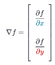
The derivative of a single variable function, denoted by f’(x) or df/dx, tells us how much the function value changes with a unit change in the input. But if a function takes multiple inputs x and y, we need to know how much the value of the function changes with respect to x and y individually i.e., how much f(x,y) changes when x changes a teeny-tiny bit while keeping y constant and also how much it changes when y changes a teeny-tiny bit while keeping x constant. These are called partial derivatives of the function often denoted by ∂f/∂x and ∂f/∂y respectively and when you put these two innocent scalars in a vector, denoted by ∇f, like the following, you get what we call the hero of calculus, the gradient!!
There are many more properties but let us just focus on two necessary ones:
The first property says that if you imagine standing at a point (x, y) in the input space of f, the vector ∇f(x, y) tells you which direction you should travel to increase the value of f most rapidly. This obviously generalizes to N dims. When I first learned this in school, it was not at all obvious why this would be the case, but check out these set of videos on Khan Academy to know more about this.
To understand the second property, we need to know what a derivate is, visually. The derivate of a line is the slope of the line, the derivative of a curve at any point is the slope of the tangent to that curve at that point.
For functions of two variables (a surface), there are many lines tangent to the surface at a given point. If we have a nice enough function, all of these lines form a plane called the tangent plane to the surface at the point.
I am sure you can convince yourself that this plane at the maximum of the surface, i.e., at the tip of the surface, will be parallel to the XY-plane Which suggests that the tangent’s slope is 0 at maximum. If you can’t, look at the following.
Arguably, the value you’d want to care about the most while training a neural network is the loss/cost. It measures how “good” or “bad” your model is fitting the data. Any GD like algorithm’s primary goal is to find the set of parameters that produce the least cost. All the drama around references like “finding the minimum,” “walking on the error surface” are just talking about adjusting the parameters in a way we end up with the least possible cost function value. You could think of a cost function as a multivariable function with model weights as the parameters. Try not to think beyond 2 parameters — you know why!
There are many ways you can frame your loss function. Different types of problems (classification & regression) can have different types of loss functions framed that best represent the performance of the models, which is for another day, another post. For now, this intuition is good enough to understand the rest of the story. You can watch this video [6] by Siraj Raval to know more about loss functions.
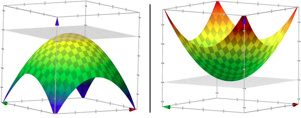
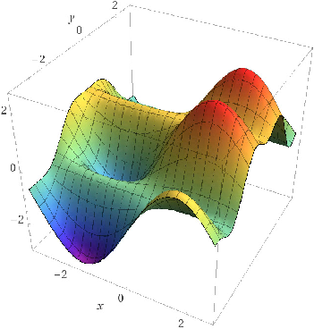
In figure 1, how many “minimums” do you see? I see just one. How nice! If your loss function looked like that, you could start your descent from anywhere on the graph (I mean, keep changing your parameters) with a reliable guide alongside (ahem Gradient Descent ahem), there is a good chance you’d end up at that sweet dark green spot on the surface. Too bad, the error surfaces you’d end up while optimizing even the smallest networks could be bumpier and in some sense, scarier.
In many real-world cases, the minimum values you are going attain depend significantly on the point at which you start the descent. If you started your descent near a valley, the GD algorithm would most definitely force you to go into that valley (a local minimum), but the real minimum (global minimum) could be somewhere else on the surface.
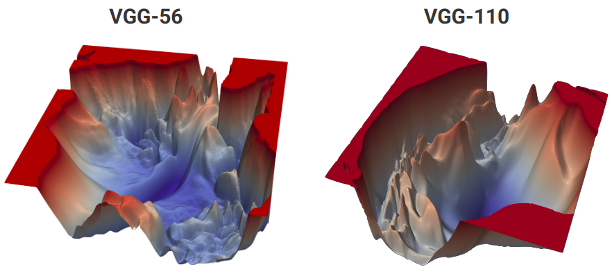
Take a look at the cost function of the two of the most popular neural networks, VGG-56 and VGG-110.
Pause and ponder!!
How can you possibly visualise a “big” network’s cost function in 3D? Big networks often have millions of parameters so how is this even possible? Read the paper linked in the references to find out.
Visualizing things in 3-D can sometimes be a bit cumbersome, and contour maps come in as a handy alternative for representing functions with 2-D input and 1-D output. It is easier to explain it graphically than in text.
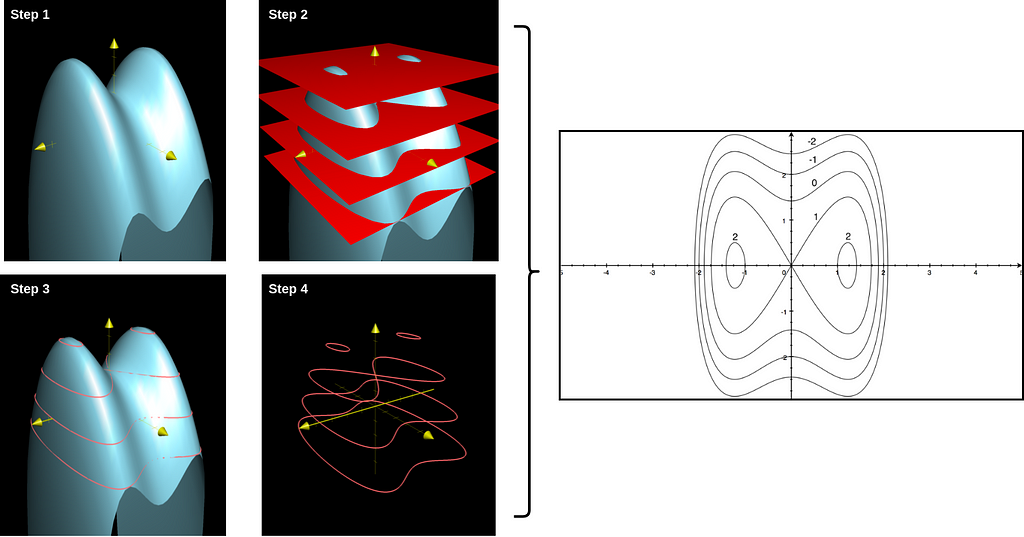
Step 1: Start with the graph of the function.
Step 2: Slice it up in regular intervals with planes parallel to the input plane at different heights.
Step 3: Mark all the places on the graph the plane cuts through.
Step 4: Project the markings on a 2-D plane, label the corresponding plane heights and map them accordingly.
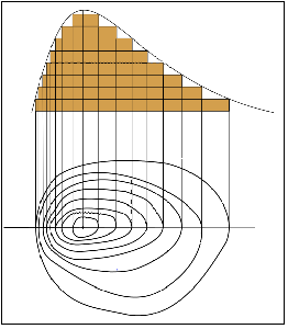
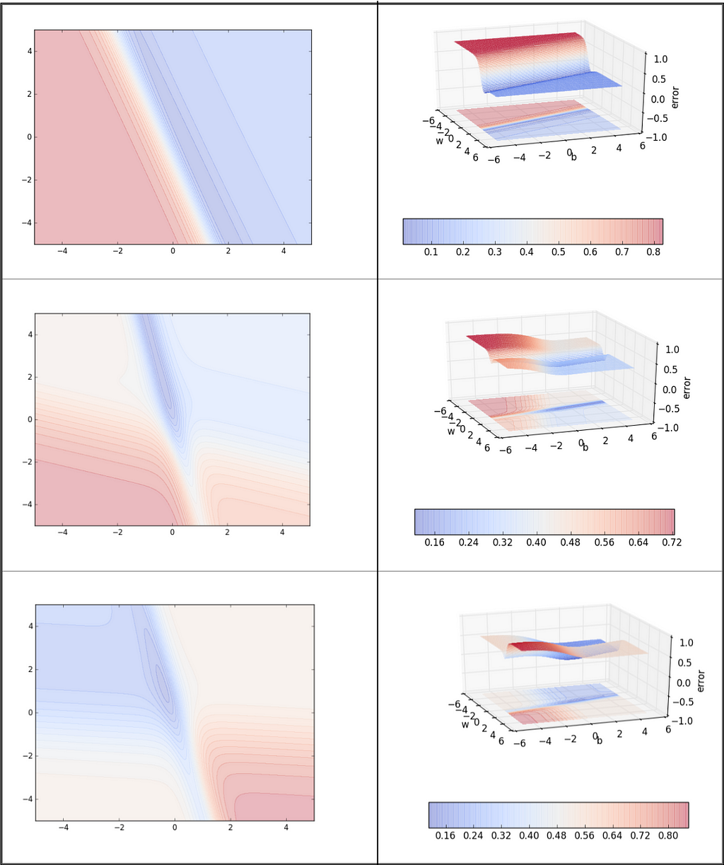
It is alright if you are still unable to comprehend the concept of contour maps completely. You can test your understanding by guessing the 3-D plots (without looking at the solution present on the right column of Figure 6) for the following contour maps.
Please read this brilliant article [7] by Khan Academy to know more about Contour Maps.
Check out the next post in this series at :
<hr><p>Learning Parameters, Part 0: Basic Stuff was originally published in TDS Archive on Medium, where people are continuing the conversation by highlighting and responding to this story.</p>