Gradient Descent is one of the most popular techniques in optimization, very commonly used in training neural networks. It is intuitive and explainable, given the right background of essential Calculus. Take a look at this blog post of mine — Part 0 of sorts, that covers some of the prerequisites needed to make better sense of this series. You can check out all the posts in the Learning Parameters series by clicking on the kicker tagged at the top of this post.
In this blog post, we build up the motivation for Gradient Descent using a toy neural network. We also derive Gradient Descent update rule from scratch and interpret what happens geometrically using the same toy neural network.
Citation Note: Most of the content and figures in this blog are directly taken from Lecture 5 of CS7015: Deep Learning course offered by Prof. Mitesh Khapra at IIT-Madras.
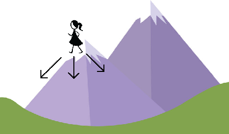
Imagine you’re standing on a mountain, there could be a lot of possible paths available to you to descend. Gradient Descent (GD) in a nutshell gives you a principled way of descending the mountain.
GD encourages you first to find a direction in which the mountain has the steepest ascent and asks you to go quite the opposite to that. You might argue that this seemingly simple idea, might not always work. You are right, GD could make you walk slow even when the surface is flat (when you can run), but we will address the limitations later at the end of the post.
Taking the metaphor forward to a toy example, let’s say we want to train a toy neural network with just one neuron. And the premise is as follows:
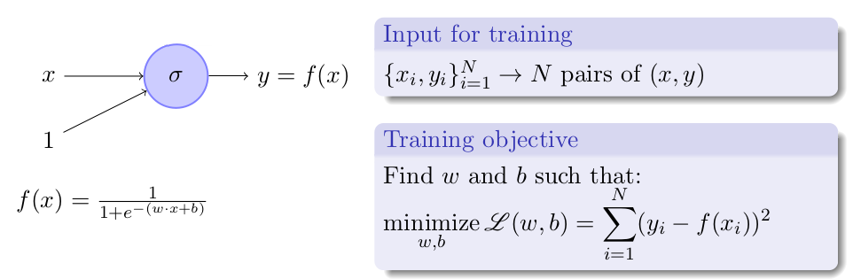
The training objective is to find the best combination of w and b that makes function L(w, b) output its minimum value.
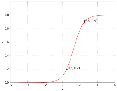
Now, what does it mean to train a network? Suppose we train the toy network with (x, y) = (0.5, 0.2) and (2.5, 0.9), at the end of the training, we expect to find w* and b* such that f(0.5) outputs 0.2 and f(2.5) outputs 0.9. We hope to see a sigmoid function such that (0.5, 0.2) and (2.5, 0.9) lie on the sigmoid.
Can we try to find such a w*, b* manually?
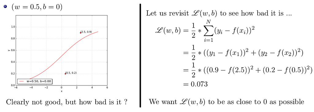
Let us try a random guess.. (say, w = 0.5, b = 0)
Let’s keep guessing. Shall we?
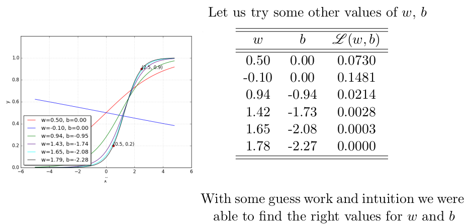
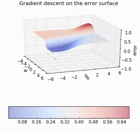
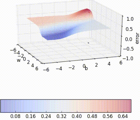
Can we visualize the guesswork? We can! Since we have only 2 points and 2 parameters (w, b) we can easily plot L(w, b) for different values of (w, b) and pick the one where L(w, b) is minimum.
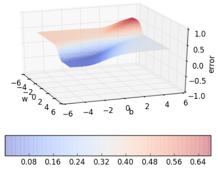
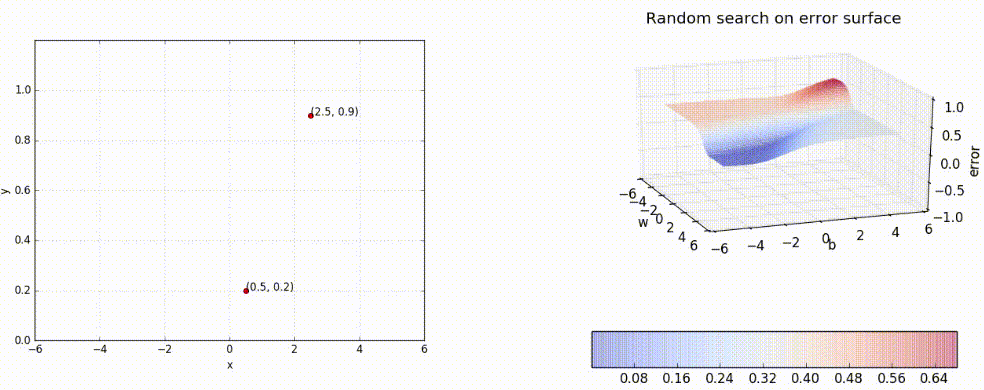
But of course, this becomes intractable once you have many more data points and many more parameters! Further, here we have plotted the error surface only for a small range of (w, b), from (−6, 6) and not from (−inf, inf). Gradient Descent to the rescue!
If it’s not already clear, the task at hand is all about finding the best combination of parameters that minimize the loss function. Gradient Descent gives us a principled way of traversing the error surface so that we can reach the minimum value quickly without resorting to brute force search.
It is reasonable to randomly initialize w and b and then update them iteratively in the best way possible to reach our goal of minimizing the loss function. Let us mathematically define this.
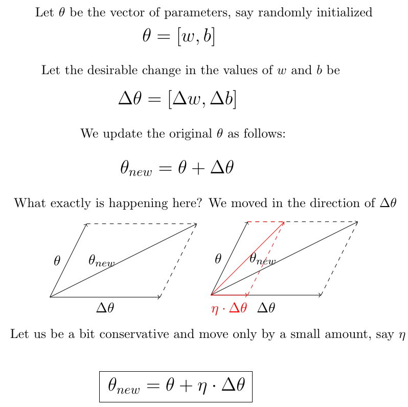
But how do we find the most ‘desirable’ change in θ? What is the right Δθ to use? The answer comes from the Taylor Series.

This means the direction u or Δθ that we intend to move in should be at 180-degree angle w.r.t. the gradient. At a given point on the loss surface, we move in the direction opposite to the gradient of the loss function at that point. This is the golden Gradient Descent Rule!!
Now that we have a more principled way of moving in the w-b plane than our brute force algorithm. Let’s create an algorithm from this rule…
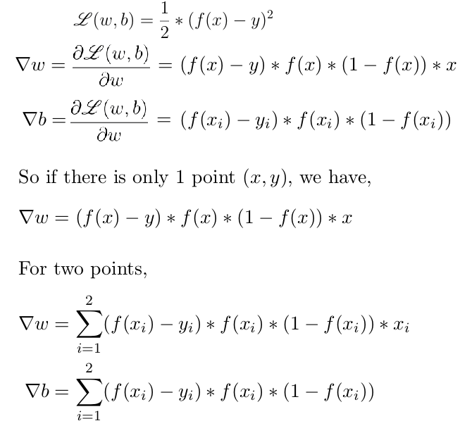
To see GD in practice, we first have to derive ∇w and ∇b for our toy neural network. If you work it out, you’ll see that they are as follows:
Let’s start from a random point on the error surface and look at the updates.
Gradient Descent in its raw form has an obvious drawback. Let look at an example curve f(x) = x² + 1, shown below:
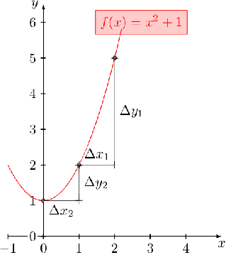
Recall that our weight updates are proportional to the gradient w = w — η∇w. Hence, in the regions where the curve is gentle, the updates are small whereas in the regions where the curve is steep the updates are large. Let’s see what happens when we start from a different point on the surface.
Irrespective of where we start from, once we hit a surface which has a gentle slope, the progress slows down. Due to this, training methods could take forever to converge.
In this blog post, we made an argument to emphasize on the need of Gradient Descent using a toy neural network. We also derived Gradient Descent update rule from scratch and interpreted what goes on with each update geometrically using the same toy neural network. We also addressed a significant limitation of GD, issue of slowing down at gentle regions, in its raw form with a curve illustration. Momentum-Based Gradient Descent overcomes this drawback to an extent by letting the ‘momentum’ of recent gradient updates control the update magnitude in the current step.
Read all about it in the next post of this series at:
A lot of credit goes to Prof. Mitesh M Khapra and the TAs of CS7015: Deep Learning course by IIT Madras for such rich content and creative visualizations. I merely just compiled the provided lecture notes and lecture videos concisely.
<hr><p>Learning Parameters, Part 1: Gradient Descent was originally published in TDS Archive on Medium, where people are continuing the conversation by highlighting and responding to this story.</p>