
In this post, we look at how the gentle-surface limitation of Gradient Descent can be overcome using the concept of momentum to some extent. Make sure you check out my blog post — Learning Parameters, Part-1: Gradient Descent, if you are unclear of what this is about. Throughout the blog post, we work with the same toy problem introduced in part-1. You can check out all the posts in the Learning Parameters series by clicking on the kicker tag at the top of this post.
In part-1, we saw a clear illustration of a curve where the gradient can be small in gentle regions of the error surface, and this could slow things down. Let’s look at what momentum has to offer overcome this drawback.
Citation Note: Most of the content and figures in this blog are directly taken from Lecture 5 of CS7015: Deep Learning course offered by Prof. Mitesh Khapra at IIT-Madras.
The intuition behind MBGD from the mountaineer’s perspective (yes the same trite metaphor we used in part-1) is
If I am repeatedly being asked to move in the same direction then I should probably gain some confidence and start taking bigger steps in that direction. Just as a ball gains momentum while rolling down a slope.
We accommodate the momentum concept in the gradient update rule as follows:
In addition to the current update, we also look at the history of updates. I encourage you to take your time to process the new update rule and try and put it on paper how the update term changes in every step. Or keep reading. Breaking it down we get
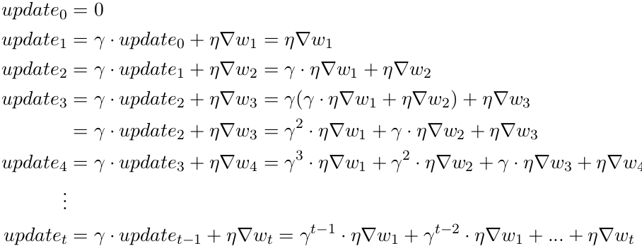
You can see that the current update is proportional to not just the present gradient but also gradients of previous steps, although their contribution reduces every time step by γ(gamma) times. And that is how we boost the magnitude of the update at gentle regions.
We modify the vanilla gradient descent code (shown in Part-1 & also available here) a little bit as follows:
From now on, we will only work with contour maps. Visualizing things in 3-D can be cumbersome, so contour maps come in as a handy alternative for representing functions with 2-D input and 1-D output. If you are unaware of/uncomfortable with them, please go through section 5 of my basic stuff blog post — Learning Parameters, Part-0: Basic Stuff (there is even a self-test you can take to get better at interpreting them). Let’s see how effective MBGD is using the same toy neural network we introduced in part-1.
It works. 100 iterations of vanilla gradient descent make the black patch, and it is evident that even in the regions having gentle slopes, momentum-based gradient descent can take substantial steps because the momentum carries it along.
On a critical note, is moving fast always good? Would there be a situation where momentum would cause us to overshoot and run past our goal? Let test the MBGD by changing our input data so that we end up with a different error surface.
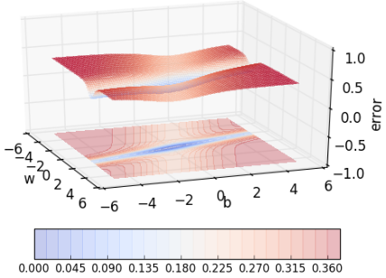
Say this one shown above, where the error is high on either side of the minima valley. Could momentum still work well in such cases or could it be detrimental instead? Let’s find out.
We can observe that momentum-based gradient descent oscillates in and out of the minima valley as the momentum carries it out of the valley. This makes us take a lot of U-turns before finally converging. Despite these U-turns, it still converges faster than vanilla gradient descent. After 100 iterations momentum-based method has reached an error of 0.00001 whereas vanilla gradient descent is still stuck at an error of 0.36.
Can we do something to reduce the oscillations/U-turns? Yes, Nesterov Accelerated Gradient Descent helps us do just that.
The intuition behind NAG can be put into a single phrase:
Look ahead before you leap!


But why would looking ahead help us in avoiding overshoots? I urge you to pause and ponder. If it’s not clear, I am sure it will be clear in the next few minutes. Take a look at this figure for a moment.
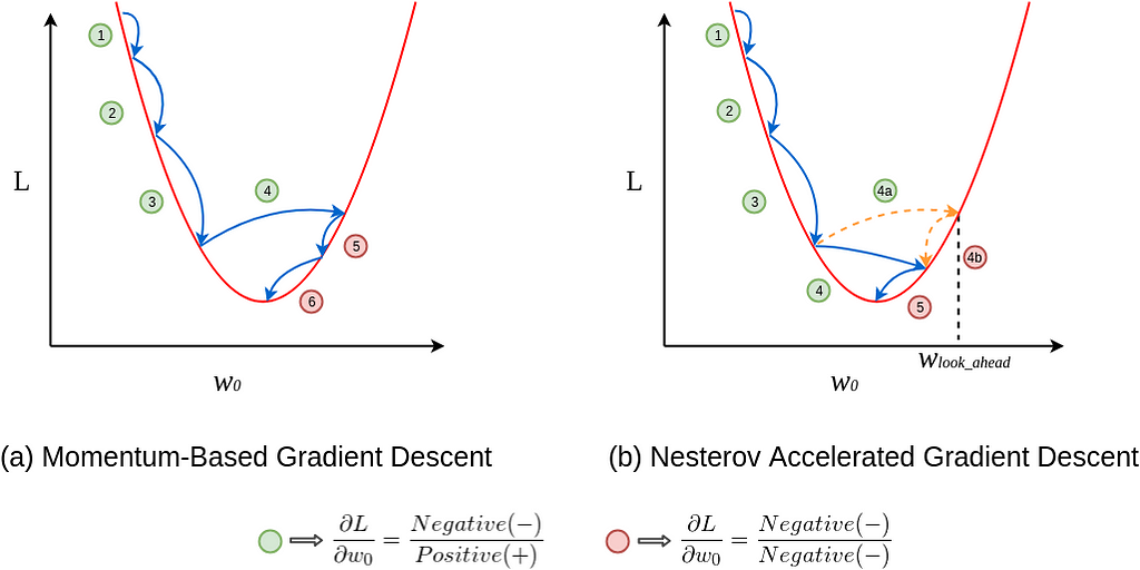
In figure (a), update 1 is positive i.e., the gradient is negative because as w_0 increases L decreases. Even update 2 is positive as well and you can see that the update is slightly larger than update 1, thanks to momentum. By now, you should be convinced that update 3 will be bigger than both update 1 and 2 simply because of momentum and the positive update history. Update 4 is where things get interesting. In vanilla momentum case, due to the positive history, the update overshoots and the descent recovers by doing negative updates.
But in NAG’s case, every update happens in two steps — first, a partial update, where we get to the look_ahead point and then the final update (see the NAG update rule), see figure (b). First 3 updates of NAG are pretty similar to the momentum-based method as both the updates (partial and final) are positive in those cases. But the real difference becomes apparent during update 4. As usual, each update happens in two stages, the partial update (4a) is positive, but the final update (4b) would be negative as the calculated gradient at w_lookahead would be negative (convince yourself by observing the graph). This negative final update slightly reduces the overall magnitude of the update, still resulting in an overshoot but a smaller one when compared to the vanilla momentum-based gradient descent. And that my friend, is how NAG helps us in reducing the overshoots, i.e. making us take shorter U-turns.
By updating the momentum code slightly to do both the partial update and the full update, we get the code for NAG.
Let’s compare the convergence of momentum-based method with NAG using the same toy example and the same error surface we used while illustrating the momentum-based method.
NAG is certainly making smaller oscillations/taking shorter U-turns even when approaching the minima valleys on the error surface. Looking ahead helps NAG in correcting its course quicker than momentum-based gradient descent. Hence the oscillations are smaller and the chances of escaping the minima valley also smaller. Earlier, we proved that looking back helps *ahem momentum ahem* and we now proved that looking ahead also helps.
In this blog post, we looked at two simple, yet hybrid versions of gradient descent that help us converge faster — Momentum-Based Gradient Descent and Nesterov Accelerated Gradient Descent (NAG) and also discussed why and where NAG beats vanilla momentum-based method. We looked at the nuances in their update rules, python code implementations of the methods and also illustrated their convergence graphically on a toy example. In the next post, we will digress a little bit and talk about stochastic versions of these algorithms.
Read all about it in the next post of this series at:
A lot of credit goes to Prof. Mitesh M Khapra and the TAs of CS7015: Deep Learning course by IIT Madras for such rich content and creative visualizations. I merely just compiled the provided lecture notes and lecture videos concisely.
<hr><p>Learning Parameters, Part 2: Momentum-Based And Nesterov Accelerated Gradient Descent was originally published in TDS Archive on Medium, where people are continuing the conversation by highlighting and responding to this story.</p>