In part 2, we looked at two useful variants of gradient descent — Momentum-Based and Nesterov Accelerated Gradient Descent. In this post, we are going to look at stochastic versions of gradient descent. You can check out all the posts in the Learning Parameters series by clicking on the kicker tag at the top of this post.
Citation Note: Most of the content and figures in this blog are directly taken from Lecture 5 of CS7015: Deep Learning course offered by Prof. Mitesh Khapra at IIT-Madras.
Let us look at vanilla gradient descent we talked about in part-1 of the series.
If you observe the block of code between the two weirdly commented lines, you notice that the gradient is calculated across the entire dataset. Meaning, the algorithm goes over the entire data once before updating the parameters. Why? Because this is the true gradient of the loss as derived earlier in part-1 (the sum of the gradients of the losses corresponding to each data point). This is a good thing as we are not approximating anything. Hence, all theoretical assumptions and guarantees hold (in other words each step guarantees that the loss will decrease). Is this desirable? Sure it is, but what is the flipside?
Imagine we have a million points in the training data. To make 1 update to w, b the algorithm makes a million calculations. Obviously, this could be very slow!! Can we do something better? Yes, let’s look at stochastic gradient descent.
Stochastic gradient descent (often shortened to SGD) is an iterative method for optimizing a differentiable objective function, a stochastic approximation of gradient descent optimization. Basically, you are going with an approximation of some sort instead of the noble ‘true gradient’. Stochastic gradient descent is the dominant method used to train deep learning models. Let’s straightaway look at the code for SGD.
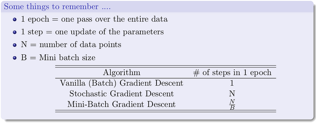
Here’s what’s going on — instead of making an update by calculating gradients for all the data points, we make an update with gradients of just one data point at a time. Thus, the name stochastic, as we are estimating the total gradient based on a single data point. Almost like tossing a coin only once and estimating P(heads). Now if we have a million data points we will make a million updates in each epoch (1 epoch = 1 pass over the data; 1 step = 1 update). What is the flipside? It is an approximate (rather stochastic) gradient so no guarantee that each step will decrease the loss.
Let us see this algorithm geometrically when we have a few data points.
If you look closely, you can see that our descent makes many tiny oscillations. Why? Because we are making greedy decisions. Each point is trying to push the parameters in a direction most favorable to it (without being aware of how this affects other points). A parameter update which is locally favorable to one point may harm other points (its almost as if the data points are competing with each other). Can we reduce the oscillations by improving our stochastic estimates of the gradient (currently estimated from just 1 data point at a time)? Yes, let’s look at mini-batch gradient descent.
In the case of mini-batch, instead of making an update with gradients of one data point at a time, we calculate gradients of a batch of data points, of size, say k. Let’s look at the code of MBGD.
Notice that the algorithm updates the parameters after it sees a mini_batch_size number of data points. The stochastic estimates should now be slightly better.
Let’s see this algorithm in action when we have k/mini_batch_size = 2.
Even with a batch size of k=2, the oscillations have reduced slightly. Why? Because we now have somewhat better estimates of the gradient (analogy: we are now tossing the coin k=2 times to estimate P(heads)). The higher the value of k, the more accurate the estimates will be. In practice, typical values of k are 16, 32, 64. Of course, there are still oscillations, and they will always be there as long as we are using an approximate gradient as opposed
to the ‘true gradient.’
The illustration isn’t clear, and on top of that the k is just 2, so it is hard to see much of a difference. But trust the math, mini-batch helps us get slightly better gradient estimates.
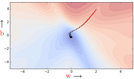
We can have stochastic versions of momentum based gradient descent and Nesterov accelerated gradient descent.

While the stochastic versions of both Momentum (red)and NAG (blue) exhibit oscillations the relative advantage of NAG over Momentum still holds (i.e., NAG takes relatively shorter u-turns). Furthermore, both of them are faster than stochastic gradient descent (after 60 steps, stochastic gradient descent [black - left figure] still exhibits a very high error whereas NAG and momentum are close to convergence).
And, of course, we can also have the mini-batch versions of Momentum and NAG but just not in this post.
In this part of the learning parameters series, we looked at variations of the gradient descent algorithm that approximate the gradients updates — Stochastic Gradient Descent and Mini-Batch Gradient Descent. We looked at the key differences between them, python code implementations of both the methods and also illustrated their convergence graphically on a toy problem. We also visualized stochastic versions of Momentum and NAG. In the next post, we will discuss a few useful tips for adjusting the learning rate and momentum related parameters and briefly look at what line search is.
Read all about it in the next post of this series at:
A lot of credit goes to Prof. Mitesh M Khapra and the TAs of CS7015: Deep Learning course by IIT Madras for such rich content and creative visualizations. I merely just compiled the provided lecture notes and lecture videos concisely.
<hr><p>Learning Parameters, Part 3: Stochastic & Mini-Batch Gradient Descent was originally published in TDS Archive on Medium, where people are continuing the conversation by highlighting and responding to this story.</p>