In part 3, we looked at stochastics and mini-batch versions of the optimizers. In this post, we will look at some commonly followed heuristics on how to tune the learning rate, etc. If you are not interested in these heuristics, feel free to skip to part 5 of the Learning Parameters series.
Citation Note: Most of the content and figures in this blog are directly taken from Lecture 5 of CS7015: Deep Learning course offered by Prof. Mitesh Khapra at IIT-Madras.
One could argue that we could have solved the problem of navigating gentle slopes by setting the learning rate high (i.e., blow up the small gradient by multiplying it with a large learning rate η). This seemingly trivial idea does sometimes work at gentle slopes of the error function, but it fails to work when the error surface is flat. Here’s an example:
Clearly, on the regions which have a steep slope, the already large gradient blows up further and the large learning rate sort of helps the cause but as soon as the error surface flattens, it doesn’t help a lot. It would be safe to assume that it is always good to have a learning rate which could adjust to the gradient and we will see a few such algorithms in the next post (part 5) in the Learning Parameters series.
Step Decay
Exponential Decay
1/t Decay
The following schedule was suggested by Sutskever et al., 2013
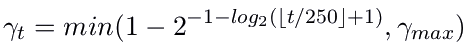
where, γ_max was chosen from {0.999, 0.995, 0.99, 0.9, 0}.
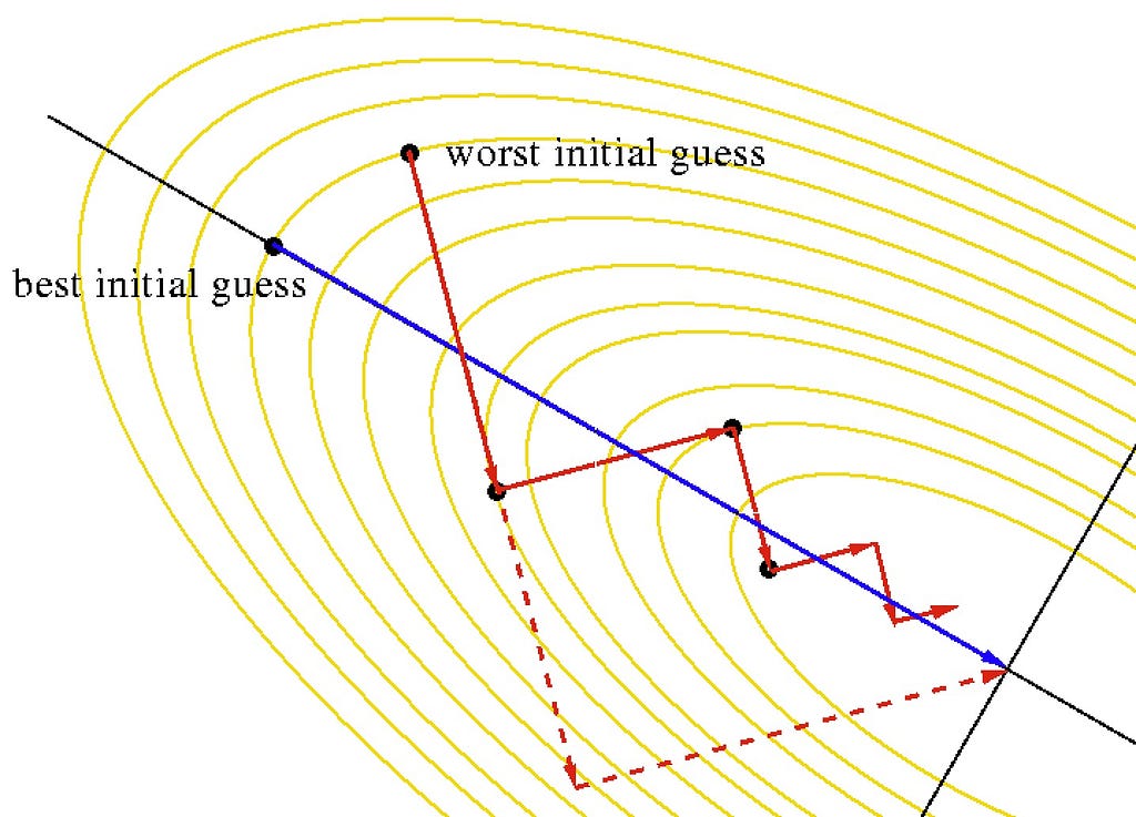
In practice, often a line search is done to find a relatively better value of η. In line search, we update w using different learning rates (η) and check the updated model’s error in every iteration. Ultimately, we retain that updated value of w which gives the lowest loss. Take a look at the code:
Essentially at each step, we are trying to use the best η value from the available choices. This is obviously not the best idea. We are doing many more computations in each step but that’s the trade-off for finding the best learning rate. Today, there are cooler ways to do this.
Clearly, convergence is faster than vanilla gradient descent (see part 1). We see some oscillations but notice that these oscillations are quite different from what we see in momentum and NAG (see part 2).
Note: Leslie N. Smith in his 2015 paper, Cyclical Learning Rates for Training Neural Networks proposed a smarter way than line search. I refer the reader to this medium post by Pavel Surmenok to read more about it.
In this part of the learning parameters series, we looked at some heuristic that can help us tune the learning rate and momentum for better training. We also looked at Line Search, a once-popular method to finding the best learning rate at every step of the gradient update. In the next (final) part of the learning parameters series, we will closely look at gradient descent with adaptive learning rate, specifically the following optimizers — AdaGrad, RMSProp, and Adam.
You can find the next part here:
A lot of credit goes to Prof. Mitesh M Khapra and the TAs of CS7015: Deep Learning course by IIT Madras for such rich content and creative visualizations. I merely just compiled the provided lecture notes and lecture videos concisely.
<hr><p>Learning Parameters Part 4: Tips For Adjusting Learning Rate, Line Search was originally published in TDS Archive on Medium, where people are continuing the conversation by highlighting and responding to this story.</p>